Appendix: Theory ¶

This section was not written for general readers. This is not intended as part of the curriculum for learning (or teaching) Bayes Theorem for day-to-day problems. The manual can be used in its entirety without reading this section. If there is any doubt in your mind, you should stop reading at this point.

This section was written for the author’s sake, to make sure he had all the details correct. It might also be helpful for technical reviewers. A few very detail oriented readers may want to peruse this section to provide some rigor for the methods shown in the rest of the manual.

Disambiguation of the language we use for probability and statistics ¶

The introduction to this manual described how probability and statistics differ in this manual. Descriptive statistics are a description of observed data and probability is a belief. Statistical inference allows us to reason about the data that we are observing to try and explain our world.

There are many classic examples - rolling dice, drawing cards, flipping coins - where you can count all the possible outcomes and interpret probability as a frequency of occurrence as the most useful way to think about the problem. These are known as frequentest probabilities. The uncertainty in these situations is a result of the process that generates the data. Given enough observations of these types of processes - say 100 coin flips - the probabilities start to converge. There might be a run of 7 heads at some point, which is curious, but eventually the ratio of heads to tails will converge.

This manual mainly uses subjective probabilities instead of frequentest probabilities. Subjective probabilities are simply opinions. Hopefully, you back your opinions up with some sort of evidence/data/logic/experience, but there is no mathematical constraint on how you derive your opinions. This lack of rigor makes subjective probabilities very helpful or very dangerous based on your level of skill. The responsibility is on you to generate probabilities that are useful to you. Bayes theorem does not care where your probabilities come from, so using either frequentest or subjective probabilities is valid. If you choose to use subjective probabilities - which we do repeatedly in this manual - you have to acknowledge that the results are personal. Someone else looking at the same data may start with a very different opinion/belief/probability and arrive at a much different result than you. This, of course, is perfectly acceptable as long as you realize there is no guarantee that your world view is correct in an absolute sense. Even with the dangers of subjective probabilities, using Bayes theorem to think about your problem means you are attempting to think critically.

For me, the more interesting set of problems is the case where the uncertainty is not in the process, but rather due to our lack of understanding. We are uncertain which candidate will win a future election, but there is no randomness in how votes are counted. Just because we lack an understanding of who will vote in any given election and how they will cast their vote doesn’t mean that elections have an element of randomness. This second type of problem can benefit from the use of Bayesian probability and is the focus of this manual.

It’s not always easy to identify what someone is talking about without context because percentages can be used for both statistics and probability. In practical cases, you need to use both statistics and probability to solve problems so being as explicit as possible with your language is important. In this manual, probabilities are represented as a decimal and never a percentage.

To further complicate the nomenclature that is being discussed, is my goal of thinking in probabilities . This is my way of saying that I think we should use statistical inference when thinking about everyday problems. The goals of statistical inference can include statistical significance, parameter estimation, prediction of data values, and model comparison. This manual focuses solely on model comparison because there are many practical applications. I often cast competing models as a hypothesis, but there is no relation to the null hypothesis testing which is commonly used in controlled experiments.

What we call things matters because it influences how we teach and describe concepts. In this manual statistics are descriptive, probabilities are beliefs, and hypotheses are models of how something works. We use Bayes theorem for inference with the goal of identifying the most likely hypothesis given the data that we have observed.

Derivation of Bayes Theorem ¶

Recall that we are investigating a very small piece of the wide world of Bayesian statistics. The derivation shown here will be limited to just the application in this manual. The end goal, is to derive the odds form of Bayes theorem. To achieve the end goal we have to settle on the notation and basic concepts for probability and odds. The basic laws of probability are taken as givens without proof in this manual. I would suggest [Kurt] as an excellent reference that derives the laws of probability from basic concepts using visual diagrams. The probability form of Bayes theorem is derived first so it can be used to derive the odds form. The odds form of Bayes theorem is used throughout the manual, see the standard solution method for details on its use. The probability form is the most common form of Bayes theorem shown in other texts, so deriving it also serves to form a baseline with other reference sources.

The log-odds form of Bayes theorem is trivial to derive from the odds form so it is included here because it has some very useful characteristics. I seriously considered using the log odds form as the basis for this manual, but ultimately didn’t because calculating logarithms in your head is not intuitive for most people.

These derivations rely on frequentest statistics! I admit that this is a bit hypocritical. I avoid the use of frequentest statistics when teaching Bayes theorem because there are not, in my opinion, many practical problems to which frequentest methods apply. I defend this decision because this is not intended to be part of the manuals curriculum and most readers will not read this section. Still, I wish I could find a more intuitive way to derive these equations without a loss of rigor.

Probability notation ¶

Bayes theorem is easy to derive assuming that you have a ubiquitous notation for Bayesian probability.

Basic notation ¶

Assume that you have three blue and one brown marble in a bag. Say you are interested in the probability that you will draw a blue marble at random from the bag. Using mathematical notation we can write the probability of drawing a blue marble as \(p(marble \space = \space blue)\) , or more simply \(p(blue)\) . The \(p(a)\) notation is shorthand for saying the probability of ‘a’ occurring. In this context ‘a’ is an event or a proposition that can occur.

Next, assume that we wanted to know the probability of drawing both a blue and brown marble with two successive draws from the bag. Replace the marbles after drawing them. The mathematical notation for this is \(p(blue,brown)\) . The \(p(a,b)\) notation is shorthand for saying the probability of ‘a’ and ‘b’ both occurring. This is also called a joint probability.

Finally, imagine that you draw a blue marble from the bag. Assume that you now want to know what the probability of drawing a brown marble without placing the blue marble back into the bag. This can be denoted as \(p(brown|blue)\) . The probability \(p(b|a)\) notation is shorthand for saying the probability of ‘b’ occurring given that ‘a’ occurs. In English this allows you to say, “what is the probability of an event occurring now that I have some information”.

Essentially in probability notation the comma (,) represents the word ‘and’, while the pipe (|) represents the word ‘given’. A complex example of this notation might be something like this: \(p(brown|blue,rain,monday)\) - meaning the probability of drawing a brown marble given that an earlier draw showed a blue marble, it is raining outside, and it is a Monday. In our example, the weather and the day of the week have no influence on the color of the marble that is drawn. So \(p(brown|blue,rain,monday)\) simplifies to \(p(brown|blue)\) because the color of marble is independent of the other (nonsense) variables.

Because it is used frequently, there is a special symbol in probability notation to represent an event not happening. The negation symbol ( \(\neg\) ) can be placed in front of a variable to indicate that the event did not occur. For example, \(p(\neg a)\) is read as the probability of event ‘a’ not occurring. Sometimes negation refers to a single event, like the opposite of a basketball team winning a game is loosing the game. Other times it can refer to any other event, such as any of the other 29 basketball teams winning the championship.

Product rule of probability ¶

The product rule of probability states that:

\[p(a,b) = p(a)p(b|a)\]

This combines the three concepts described in the basic notation section into a single relationship. The trivial case of the product rule occurs when the two events (a and b) are totally independent - like when rolling two fair six sided dice. The number showing on one die has no bearing on the other die. In this special case of rolling two dice, the product rule reduces to \(p(a,b) = p(a)p(b)\) . The probability of rolling a one on each die is 1/6. So the probability of rolling two ones is \(1/6 \times 1/6 = 1/36\) . In the case where marbles are drawn from the bag and not replaced, the conditional form of the product rule is required:

\[p(blue,brown) = p(blue)p(brown|blue)\]

With initially three blue and one brown marble in the bag \(p(blue) = 3/4\) . After drawing a blue marble out of the bag, and not replacing it, \(p(brown|blue)\) is now \(1/3\) . Putting it all together:

\[p(blue,brown) = p(blue)p(brown|blue) = 3/4 \times 1/3 = 3/12 = 1/4\]

For the sake of illustration, let’s assume that the brown marble was drawn first and then the blue marble. Repeating the calculation shows that on the first draw \(p(brown) = 1/4\) and then subsequently \(p(blue|brown) = 3/3 = 1\) . Then \(p(brown,blue) = 1/4 \times 1 = 1/4\) is the same result even though the order that the marbles were drawn was different.

Marginal probability ¶

The concept of marginal probability is complimentary to the product rule of probability. The product rule is used to calculate a joint probability such as \(p(a,b)\) . The marginal probability is used to calculate the probability of just one event, say \(p(b)\) across all of the other possible outcomes of \(a\) . The marginal probability of a joint probability is:

(2) ¶ \[ p(b) = \sum_a p(a,b) = \sum_a p(a)p(b|a) \]

The product rule was used to expand the joint probability into an easier to use form. The easiest case occurs when \(a\) is a binary event. In this simple case:

\[p(b) = p(a)p(b|a) + p(\neg a)p(b|\neg a)\]

A slightly more complex example is when \(a\) is a finite set of outcomes. For example if \(a=\{a_1,a_2,a_3\}\) then:

\[p(b) = p(a_1)p(b|a_1) + p(a_2)p(b|a_2) + p(a_3)p(b|a_3)\]

Mutually exclusive and exhaustive propositions ¶

The next two concepts - a set of mutually exclusive and exhaustive propositions - by itself seem academic. In the next section these concepts will be critical in understanding what the denominator in Bayes theorem means.

In probability notation, a set of propositions (or outcomes) are mutually exclusive if only one proposition can be true. For example, in a game maybe you can either win or loose, but never have a draw. A more complex example is the NFL draft where there are 224 total selections from a pool of approximately 3000 players . A player is either drafted to a single team or they are not. There are no other possible outcomes during the draft.

A set of propositions is exhaustive if they cover every possible outcome. Again, a win/lose game where there can be no draws is an exhaustive set. Similarly, only people who posses a lottery ticket are eligible to win the lottery.

Taken together a set of propositions are mutually exclusive and exhaustive if you can explicitly write down all the possible outcomes and be sure that only one of those outcomes will occur. In practice this can be difficult to achieve. For example, consider your typical murder mystery. The suspects might be Mr. Green, Col. Mustard, and Ms. Scarlet. In real life, it is hard to fully eliminate the tiny possibility that some other seemingly random person, like a secret agent, didn’t commit the murder.

In summary for a set \(X = \{X_1,X_2,...X_n\}\) of propositions:

Mutually exclusive means that the probability of any two events both occurring will be zero: \(p(X_i,X_j) = 0\) .
Exhaustive means the union of all propositions is one: \(p(X_1 \lor X_2 \lor...\lor X_n) =1\) . This implies that at least one of the propositions has a probability of one.
Propositions are mutually exclusive and exhaustive if the total probability of all propositions represents all possible outcomes: \(\sum_{i=1}^{n}p(X_i)=1\) .

The special case of binary events ¶

Binary events, where there are only two possible outcomes, are a special case in probability theory. This manual uses this special case extensively because the math is easier when you constrain the solution process to binary events. There are plenty of other ways to apply Bayes theorem when not analyzing a binary event, but those methods are mostly beyond the scope of this manual.

True/false, fake/real, success/failure, win/lose, honest/corrupt, etc. are examples of binary events. If you can say that some proposition, a, is a binary event, then \(p(a) + p(\neg a) = 1\) . This also implies that the set \(\{a,\neg a\}\) is mutually exclusive and exhaustive. In this special case \(\neg a\) is a mutually exclusive event instead of a catch all for ‘everything else that could happen’.

Probability form of Bayes theorem ¶

Bayes theorem is derived by using the product rule of probability. If \(p(a,b)\) is stating the probability that both events ‘a’ and ‘b’ occur, then the order the variables are written in should not matter.

\[p(a,b) = p(b,a)\]

This expands via the product rule to:

\[p(a)p(b|a) = p(b)p(a|b)\]

Dividing through by \(p(b)\) results in the commonly shown form of:

(3) ¶ \[ p(a|b) = \frac{p(a)p(b|a)}{p(b)} \]

As far as I can tell, \(p(a|b) = p(a)p(b|a)/p(b)\) is the most general form of Bayes theorem, but also not directly applicable to many real world problems. To actually use the formula you have to make an assumption and expand (or neglect!) the denominator. Also, you usually have to assume how many possible states of the world you are willing to consider. Some of the common situations are:

One hypothesis, two possible outcomes
Multiple hypothesis, two possible outcomes
Multiple hypothesis, multiple possible states
Continuous range of hypotheses and states

In this manual, we primarily concern ourselves with the first two situations. The math is much simpler when you constrain the problem to a binary outcome (true/false, success/fail, etc.). In practice, many problems can be cast as a binary outcome so this is not a significant constraint. If your problem can’t be cast as a binary event then you can always use a more complex form of Bayes theorem, see parameter estimation for a glimpse of how this works.

Application specific notation ¶

The form used through much of this manual is the odds form of Bayes theorem. It is derived from the above general form using a couple of simplifying assumptions. The first assumption is that we are choosing to use Bayes theorem for hypothesis testing or model comparison. What is shown here won’t work for parameter estimation problems. To break away from the general case to a more specific case, substitute in more meaningful variable names. Recast the theorem derived above in terms of the variable names hypothesis (H) and evidence (e):

(4) ¶ \[ p(H|e) = \frac{ p(H)p(e|H)}{p(e)} \]

I like to use the notation hypothesis instead of model because a model tends to be a formal thing - like a weather model. By comparison, a hypothesis can be very informal, like ‘I believe Mr Green is the murderer’, or ‘I believe that an acquaintance is jealous’. If you have a complex and rigorous hypothesis that is great, but less rigorous hypotheses will work as well.

In the new notation, evidence is a general term for anything that is known because of observation. Similar to a hypothesis, evidence can come in many forms ranging from cold hard data to gossip at the water cooler. Evidence can be generated in many ways, for example:

Totally unplanned observations that you just happened to be lucky enough to see
The result of research into existing data sets
The outcome of a controlled experiment
Purchasing advice from a expert

Bayes theorem will help us weigh the strength of the evidence so we can modify our beliefs. Evidence with little to no strength will have have little to no impact on our beliefs.

By convention, the terms in Bayes theorem are given names. I don’t like these names, but they are ubiquitous in the literature on Bayes theorem. The descriptions presented here are tailored to using the theorem for a binary event. There can be other interpretations.

\(p(H)\) : The probability of the hypothesis being true. This is known as the prior probability . Before you observed the evidence, this is what you would have believed.
\(p(e|H)\) : The likelihood of the hypothesis generating the evidence. Known simply as the likelihood . This term quantifies the strength of the evidence. This is a conditional probability that is the inverse of what we are trying to calculate.
\(p(H|e)\) : The probability of the hypothesis given the evidence. This is known as the posterior probability and is also a conditional probability. It is usually not possible to calculate this probability from the evidence unless you use Bayes theorem.

Tellingly \(p(e)\) , the denominator in the theorem, is not given a standard name by convention. The probability of the evidence is not a very intuitive concept and warrants its own section for discussion.

Probability of the evidence ¶

The derivation of the probability form of Bayes theorem is trivial if you understand the notation used. Understanding the meaning of the denominator in the theorem is where most of the complexity arises and makes the application of Bayes theorem tricky in practical situations. The odds form of Bayes theorem sidesteps this complication, which is why it is used through out this manual. To motivate why the odds form is easier to work with, we will describe some of the aspects of the denominator in the probability form of Bayes theorem.

The probability of the evidence in the denominator of Bayes theorem can be recast in terms of probabilities that we know using the marginal probability of a joint probability . Equation (5) shows equation (2) in terms of the variable names hypothesis (H) and evidence (e):.

(5) ¶ \[ p(e) = \sum_H p(H,e) = \sum_H p(H)p(e|H) \]

Therefore, Bayes theorem can be written as:

\[ p(H|e) = \frac{p(H)p(e|H)}{p(e)} = \frac{p(H)p(e|H)}{\sum_H{p(H)p(e|H)}} \]

By recasting the denominator in this way, we get to work with familiar terms, but it still can be very difficult to figure out the probability for each element in the sum found in the denominator.

We avoid continuous random variables like the plague in this manual. But, if you were to consider such situations, the sum becomes an integral and the probabilities become distributions.

(6) ¶ \[ p(H|e) = \frac{p(H)p(e|H)}{\int{p(H)p(e|H)}dH} \]

This is the most complex formulation of Bayes theorem and soon after it is presented there is usually a note saying that the calculation of the integral is impossible in practical real world situations. This always lead me to wonder why if you can’t calculate the integral, would you show the result in the first place? Most books on Bayes theorem - including this one - focus on how to exploit a loop hole of some kind so you don’t have to calculate the impossible integral.

Temporal sequencing ¶

It is important to point out that the derivation assumes no temporal sequencing of any kind. It is totally valid to observe data first and then generate a hypothesis. I believe that this is quite common in practice and makes Bayes theorem very useful. For example, evidence occurs before the hypothesis in these types of situations:

You are playing a game of chance at a casino and you lose 5 times in row, what are the odds that the casino is cheating you given your losing streak?
You find an pair of underwear that is not yours in your bedroom, what are the odds that your partner is not being faithful?
You observe an unidentified flying object (UFO), what are the odds the vehicle was extraterrestrial life?
Late October polling results show a political candidate leading in key battle ground states, what are the odds that candidate wins an early November election?
You hear a customer ask if you have fork handles , what are the odds they are really asking for four candles ?

For those familiar with the scientific method, this may sound sacrilege. Many of us are taught that good science necessitates the creation of a hypothesis first, then you test that hypothesis. If your goal is to prove something scientifically, then I couldn’t agree more with the hypothesis-then-test approach. You most often see this approach in a controlled laboratory setting. Bayes theorem can be useful in a controlled laboratory setting. However, traditional null hypothesis significance testing is also useful in a controlled laboratory setting. Applying Bayes theorem for controlled laboratory settings requires some nuance that is beyond the scope of this manual.

If your goal is to simply draw a reasonable explanation for the evidence you are observing when you are more or less naive to the underlying mechanisms, the evidence-then-hypothesis approach is perfectly acceptable.

The point is that we apply temporal constraints to Bayes theorem to fit our needs. There is nothing in the derivation that restricts the use of Bayes theorem in other ways. The use of prior and posterior makes it seem like there is a temporal order, but that is just a convention separate from the actual derivation. It is unusual, but it is even possible to work backwards from a posterior probability to identify the implied prior probability.

I personally feel that in the past I have relied too heavily on the scientific method and controlled experiments and failed to incorporate “free” evidence that happened outside the confines of the laboratory. I strongly suggest not excluding either the hypothesis-then-test or evidence-then-hypothesis approach, but rather using them together.

Odds notation ¶

The odds form of Bayes theorem is also easy to derive assuming that you have a ubiquitous notation for for the concept of relative odds and understand how they relate to probability.

A very brief history of odds and gambling ¶

The concept of odds predates the concept of probability. It will be shown that odds are typically a more user friendly way to quantify a belief, and that probability is a mathematical construct that makes derivations and proofs easier.

Given its long history, and association with gambling, the word odds is commonly used in popular speech. Specifically, exclaiming “what are the odds of that happening!” when you are surprised by something is common. Math uses common words as technical terms , so the sentence above abuses the mathematical definition used in this manual in multiple ways.

Odds in the betting world come in many forms - British, European, American moneyline - that vary across the type of game played and where in the world the betting house is located. The various betting notations are not used in this manual. Odds are a convenient way to quantify belief because it is easy to calculate the payout on a bet.

If you know the odds, you can calculate the implied probability. If you add up the implied probabilities from a bookmaker for an event, you will discover that they don’t quite sum to 1. This is of course how bookies make their money. Many people commonly bet without knowledge of the implied probability, but that is a topic for a different book…

Probability theory is intricately linked to gambling. Initially, probability theory was considered a dirty science due to its initial association with gambling. Only later when applications in the financial and insurance industries demonstrated its utility did it become a serious topic that professional mathematicians would study.

To avoid confusion with the historical meaning of odds, this manual uses the term relative odds to denote a belief. For brevity, relative odds will often be shortened to just odds in this manual.

Relative odds ¶

Relative odds are defined as a ratio, where probabilities are defined as a fraction of the whole.

In the simple case shown in Fig. 6 , probability and odds are compared. Fig. 6 shows a binary example which is a special case that makes the math easier. Colon notation (:) is used to represent the relative odds, and is pronounced as ‘to’. For example, the odds in favor of an event occurring are 3:2 or ‘three to two’. For consistency, colon notation will be used in this manual. Equivalent notations represent odds as ratios or decimals. For example, \(3:2 \Rightarrow 3/2 = 1.5\) .

Relative odds tell you how many times more likely one event is than another. If the odds for an event are 3:2, then the event is \(3/2 = 1.5\) times more likely to occur than its compliment. For example if the New Hampshire Pineapples are favored 3:2 to beat the Baltimore Nordiques, then the Pineapples are 1.5 times more likely to win 1 .

Fig. 6 Comparison of odds to probability. Source (CC-BY-SA-4.0). ¶

In the more general case, relative odds can be used to define the relative belief that a set of propositions will occur. For example, a list of murder suspects can be assigned relative odds. The odds of suspects Mr. Green, Col. Mustard, and Ms. Scarlet being the murderer might be 1:3:5 respectively 2 . In this case Col. Mustard is \(3/1=3\) times as likely to be the murderer as Mr. Green and \(3/5 = 0.6\) times as likely as Ms. Scarlet to be the murderer. Similar statements could be made comparing the other suspects.

Formally, a set of propositions (or possible outcomes to an event) can be explicitly listed as \(X = \{X_1,X_2,...,X_n\}\) . The relative odds of those propositions occurring are then \(x = \{x_1,x_2,...,x_n\}\) . Odds are ratios, so scaling a set of odds does not change its meaning. For example if \(\beta\) is a constant then for all \(n\) , such that \(y_n = \beta x_n\) , then \(x\) and \(y\) would be equivalent sets of odds. Let the odds function, \(O()\) , map a set of propositions into a set of odds: \(O(X) = x\) . Because odds can be scaled without changing their meaning, we can only go so far as to say that odds are proportional to their respective probability:

\[O(X) \propto p(X)\]

For example, if the probability of Mr. Green, Col. Mustard, and Ms. Scarlet being the murder is \(X = \{0.1,0.3,0.5\}\) respectively, then we can calculate the relative odds. Note that the probability does not sum to one in this example. This implies that we do not have an exhaustive set of propositions. Based on the given probabilities the relative odds of each suspect being the murderer are \( x_n = \{0.1,0.3,0.5\}\) which can be scaled to the friendlier form of \(\{1,3,5\}\) . If we were not being formal we could also write this with colon notation as \(1:3:5\) . Because odds can be scaled we could have also started with probabilities of \(\{0.05,0.15,0.25\}\) . This second variation is quite a different situations. The total probability that one of the suspects is the murderer is only 0.45. There is a lot of probability reserved for other, yet to be named, suspects. Somewhat misleadingly the odds are the same in both cases.

Warning

Unless you have a mutually exclusive and exhaustive set of propositions, you can not calculate probabilities from the relative odds.

If, and only if, you have a mutually exclusive and exhaustive set of propositions, then probabilities can be calculated from the odds by normalizing each element like this:

\[ \Bigg\{\frac{x_1}{\sum_{n=1}^{i}x_i},\frac{x_2}{\sum_{n=1}^{i}x_i},...,\frac{x_n}{\sum_{n=1}^{i} x_i}\Bigg\} = \{p(X_1),p(X_2),...,p(X_n)\} = p(X) \]

For the special case of binary events, which are used often in this manual, there are some simple relations to convert between odds and probability. If we let \(H_1\) and \(H_2\) be complementary events such that \(H=\{H_1,H_2\}\) then we can state that \(p(H_1) = 1 - p(H_2)\) . This allows us to easily switch back and forth between the odds and probability forms:

If \(p(H_n) = p \Rightarrow O(H_n) = \frac{p}{1-p}\)

If \(O(H_n) = q \Rightarrow p(H_n) = \frac{q}{1+q}\)

Unlike probability, which is defined on the range \([0,1]\) , odds are defined on the range \([0,+\infty]\) , which can make interpretation more difficult. Table 29 provides rough guidance on how to interpret odds, which was taken from [Kurt] . Colon notation ( \(a:b\) ) doesn’t work well when showing ranges of values in a chart, so the equivalent odds ratio ( \(a/b\) ) can be used instead.

Table 29 Guidance for interpreting odds ¶
Odds ratio ( \(a:b \Rightarrow a/b\) )	Strength of evidence
1 - 3	Interesting, but not conclusive
3 - 20	Looks like we are on to something
20 - 150	Strong evidence
>150	Overwhelming evidence

Multiplication of sets of odds is very straight forward. Multiplication is element wise. For example, if you have two separate sets of odds denoted as \(x\) and \(y\) , then \(xy=\{x_1y_1,x_2y_2,...,x_ny_n\}\) . This result will be used extensively in the odds form of Bayes theorem.

Odds form of Bayes theorem ¶

After the hard work of narrowly defining the nomenclature that we use for Bayes theorem, the derivation of the odds form is again relatively easy. Assume that you have two competing hypothesis, \(H_1\) and \(H_2\) , and you observe a single piece of evidence, \(e\) . In this manual, the competing hypothesis are most likely a binary outcome such as \(H_1\) represents true and \(H_2\) represents false. Other combinations include fake/real, win/lose, honest/corrupt, etc. It will be shown later how to extended this method to three or more hypothesis. Using the probability form of Bayes theorem from equation (4) , the probability of a hypothesis being true can be written for each hypothesis.

\[ p(H_1|e) = p(H_1)p(e|H_1)/p(e) \]

\[ p(H_2|e) = p(H_2)p(e|H_2)/p(e) \]

Dividing the two equations by each other eliminates \(p(e)\) because the same evidence is being observed for both hypothesis:

\[\frac{p(H_1|e)}{p(H_2|e)} = \frac{p(H_1)p(e|H_1)/p(e)}{p(H_2)p(e|H_2)/p(e)} = \frac{p(H_1)p(e|H_1)}{p(H_2)p(e|H_2)}\]

Separate the terms to make the result more readable:

(7) ¶ \[ \frac{p(H_1|e)}{p(H_2|e)} = \frac{p(H_1)}{p(H_2)}\times\frac{p(e|H_1)}{p(e|H_2)} \]

This intermediate step is known as the proportional form of Bayes theorem. In English, this means that the ratio of the posterior probabilities are equal to the ratio of the prior probabilities times the ratio of the likelihoods. Ratios of probabilities are relative odds. If we use the notation \(H=\{H_1,H_2\}\) and the odds function, \(O()\) , then the result can be cast like this

(8) ¶ \[ O(H|e) = O(H) \times L(e) \]

Note that \(L(e)\) gives a special designation given to the term \(p(e|H_1)/p(e|H_2)\) , known as the relative likelihood. Without mathematical notation, this result can be stated verbally as:

\[posterior \space odds = prior \space odds \times relative \space likelihood\]

Expanding each term into its respective set shows how simple a calculation with the odds form of Bayes theorem can be

\[\begin{split} \begin{align*} H &= \{H_1,H_2\}\\ O(H) &= \{h_1,h_2\}\\ L(e) &= \{l_1,l_2\}\\ O(H|e) &= \{h_1l_1,h_2l_2\} \end{align*} \end{split}\]

Again, following convention, each term is assigned a name in Bayes theorem. The mapping of the terms from the probability to odds form are not exactly one to one, so they are shown again for odds notation.

Prior odds : \(O(H)\) - This term represents what you would have thought prior to making any observations. For example, if you have a loving and healthy relationship with your partner, your prior odds that they would cheat on you would be very low. In our Worcestershire cola example, before we read the article, we were very skeptical of the headline and assigned our prior odds as very strongly in favor of fake news. In most cases, your prior odds are not an exhaustive set.

Relative likelihoods : \(L(e)\) - This term can be considered the strength of the evidence/data/research/argument. If your best friend in the world tells you your goldfish is dead then there is a strong likelihood that the goldfish is in fact dead. If a supermarket tabloid tells you that the president is a cross dressing martian, you might find it unconvincing evidence given the source and therefore a weak likelihood. While the prior odds are often based on your gut feeling, the relative likelihood is based on any additional information you are able to collect and the strength of the evidence.

Posterior odds : \(O(H|e)\) - This term is the output of Bayes theorem. This represents the odds of an event occurring given the available evidence. The posterior odds are a combination of our original belief and the strength of the evidence. The strength of your revised beliefs after observing the evidence can be evaluated using Table 29 .

Because the odds form of Bayes theorem uses element wise multiplication, it can easily be extended to accommodate a finite number of competing hypothesis simply by expanding the set of hypothesis like \(H=\{H_1,H_2,...,H_n\}\) .

Revisiting the mystic seer example ¶

I find the explanation for the likelihood in the mystic seer example to be unsatisfying because it relies on probabilities and not relative odds. Recall the that evidence in this case is seven consecutive observations of a correct answer where the probability of a correct answer is 0.5. Therefore, the likelihood using probabilities is calculated as \((0.5)^7 = 1/128 = 0.0078125\) .

Here is another way to think about the likelihood that highlights the power of sequential Bayesian updating (aka multiple belief revision 3 ).

Assume that you are one of the characters in the mystic seer example and that you are revising your beliefs after the mystic seer answers each question instead of waiting until all seven answers are provided. New evidence is generated after each answer, so to help differentiate the pieces of evidence label each observation as \(e_n\) . So \(e_1\) is the first correct answer, \(e_2\) is the next correct answer, and so on until, until seventh correct answer which will be \(e_7\) .

After the first correct answer from the seer, you could ask yourself, given each hypothesis what is the probability of observing this data. \(H_1\) represents the mystic seer being a perfect fortune teller, so you would expect the answer to be correct every time, or a probability of 1. \(H_2\) represents the hypothesis that the mystic seer is randomly guessing at the answerers. In this case, the probability of a correct answer would be 0.5. Your relative likelihood would be:

\[\frac{p(H_1|e_1)}{p(H_2|e_1)} = \frac{1}{\frac{1}{2}}=2\]

Similarly, after observing the second correct answer the relative likelihood of just that observation would be:

\[\frac{p(H_1|e_2)}{p(H_2|e_2)} = \frac{1}{\frac{1}{2}}=2\]

Taking both of the observations together results in just multiplying the likelihoods from each respective observation.

\[\frac{p(H_1|e_1, e_2)}{p(H_2|e_1, e_2)} = \frac{p(H_1|e_1)}{p(H_2|e_1)} \times \frac{p(H_1|e_2)}{p(H_2|e_2)} = \frac{1}{\frac{1}{2}} \times \frac{1}{\frac{1}{2}} = 2 \times 2 = 4\]

Continuing this argument in a similar way for each of the seven observations leads to the relative likelihood of:

\[\frac{p(H_1|e_1,e_2,e_3,...,e_7)}{p(H_2|e_1,e_2,e_3,...,e_7)} = 2 \times 2 \times 2 \times 2 \times 2 \times 2 \times 2 = 2^7 = 128\]

Previously the relative likelihood using probabilities was given as \(1:(0.5)^7 = 1:0.0078125 = 1/0.0078125 = 128\) , so the results are equivalent. I personally just like thinking with odds rather than probability. This also highlights how the strength of evidence is just multiplied together when using the odds form of Bayes theorem.

Log odds form ¶

The log-odds form of Bayes theorem is a simple transformation of the odds form of Bayes theorem shown in equation (8) . Before we start the derivation recall the property of logarithms that states:

\[log(xy)=log(x)+log(y)\]

Taking the base 2 logarithm of each side of the odds form of Bayes theorem, shown in equation (8) , results in evidence updating the prior beliefs via addition instead of multiplication.

(9) ¶ \[ log_2 \big( O(H|e) \big) = log_2 \big(O(H) \big) + log_2 \big( L(e) \big) \]

In the remainder of this section, relative odds and odds ratios will be used interchangeably so that the logarithms can be calculated. Recall that relative odds of \(a:b\) have an odds ratio of \(a/b\) .

For example, if you set your prior odds that a medical news story is real:fake at 1:128, then you then observe the following evidence (see the medical heuristic example):

Study results are published in a journal article
The study used a large number of participants
Multiple hospitals/doctors participated
The study lasted multiple years
The authors are from a well known medical school
The effect was large and statistically significant

Use a heuristic, originally suggested by Jeff Leek, where each bit of evidence doubles the likelihood that the story is real. Every bit of evidence that refutes the story haves the likelihood. All our evidence supports the news story being real, so in this case the heuristic is \(2 \times 2 \times 2 \times 2 \times 2 \times 2 \times = 2^6 = 64\) , or 64:1 in support of the story being real. Note that \(log_2(2)=1\) , so each bit of evidence adds one to the log of the posterior odds. In our example \(log_2(64) = 6\) . By virtue of how we set up the problem, positive bits imply a belief that the news story is real and negative bits imply a belief that the story is fake. Putting it all together, a summary of the problem is shown in Table 30 :

Table 30 A summary of the medical heuristic example using log odds. ¶
	Real	Fake	\(log_2(\frac{Real}{Fake})\)
Prior odds	1	128	-7
Likelihood	64	1	+6
Posterior odds	64	128	-1
Simplified posterior odds	1	2	-1

The log of the posterior odds is calculated as \(-7+6=-1\) . Because of the way we set up the problem, with odds as real:fake, this implies that you should believe that the story is fake with log-odds of -1 bit, or equivalently odds of 1:2. Initially, you believed very strongly that the story was fake. After updating, you still believe the story is fake, just with much less certainty than you initially had.

Log-odds is defined on the interval \([-\infty, +\infty]\) . By comparison, the intervals for the other forms are, probability \([0,1]\) , odds \([0,+\infty]\) , and odds ratio \([0,+\infty]\) . The \([-\infty, +\infty]\) interval in the log odds form has the desirable characteristic that high or low probabilities don’t get smashed at the ends of the interval. Unlike the other forms, doubling your belief in the log-odds always results in a change of 1 bit. Take for example revising your beliefs from 2:1 to 128:1 in increments based on increasingly convincing evidence. Table 31 compares the numerical values for the different forms of quantifying belief.

Table 31 Comparison of increasingly convincing beliefs on different intervals ¶
Odds	Probability	Odds Ratio	Log Odds	Strength of Evidence
2:1	0.67	2	+1	Interesting, but not conclusive
8:1	0.89	8	+3	Looks like we are on to something
32:1	0.97	32	+5	Strong evidence
128:1	0.99	128	+7	Almost overwhelming evidence

As a belief becomes increasingly convincing, the change in the probability interval becomes very small. For example, as a belief goes from 32:1 to 128:1 the probability index only changes by \(128/129 - 32/33 = 0.02\) . By comparison, as a belief goes from 2:1 to 8:1, the probability index changed by \(8/9-2/3 = 0.22\) . The probability index is non-linear, the impact of this is most extreme at the ends of the index near zero or one. Long shot, and near certain, probabilities are common in settings where risk is being evaluated. So the difference between risky and really risky might be only a small change in the probability index.

The odds, and therefore odds ratio, simply increase linearly as the odds change. This avoids the non linearity at the ends of the intervals near zero and one. The infinite index can make interpretation difficult because all the values are now relative. Heuristics like Table 29 , describing the strength of evidence, is a result of the shortcoming of an infinite index. Reasoning with very small odds is still not great because the numbers become very small. The index is linear with small odds, but humans don’t naturally deal with multiple decimal places well. When odds are small, the ratio can be turned around to get a feel for the magnitude of the belief, but then you have to remember to revert the odds back which is problematic.

The log-odds index, not surprisingly, is linear. Each change in belief listed in Table 32 changes the belief by 2 bits. This can be a very intuitive way to think about the strength of evidence. Manipulating bits with mental math is similarly easy, it just requires addition. There are two issues with using bits:

The practical issue with bits and the log scale is the need to take the inverse of the logarithm to get back to a traditional index. In theory, you could calibrate yourself to reason with bits. I however, still find value with sometimes using, or communicating, with the probability or odds index.
Bits are good when you constrain your likelihoods to multiples of two (…4,2,1/2,1/4…). The mental math gets more complex when you need to use a likelihood such as \(2:3 \Rightarrow log_2(2/3)=-0.58\) . The context of the problem dictates if using easy likelihoods will impact the accuracy of your reasoning in a meaningful way.

In summary, all of the indexes used to describe a belief have pros and cons. The odds index defined on \([0,+\infty]\) was chosen for this manual because it seems to represent a middle ground and involves manipulating whole numbers. Your mileage will vary with each index, and its accompanying form of Bayes theorem. The good news is that all three forms are valid if your use case warrants it.

For reference, Table 32 is Table 29 updated with the equivalent bits of evidence for comparison.

Table 32 Guidance for interpreting log odds ¶
Odds ratio	Bits	Strength of evidence
1 - 3	0 - 1.6	Interesting, but not conclusive
3 - 20	1.6 - 4.3	Looks like we are on to something
20 - 150	4.3 - 7.2	Strong evidence
>150	>7.2	Overwhelming evidence

The interplay between the prior and the relative likelihood ¶

The odds form of Bayes theorem is very simple with the only two inputs being the prior odds and relative likelihoods. If we classify these inputs as normal or extreme 4 , then we can intuitively guess what the posterior odds will be, or more importantly what the inputs need to be to modify our beliefs in a meaningful way. For this section, normal means the prior odds ratio, or the relative likelihood ratio, is less than or equal to 150. Extreme odds/likelihoods have ratios greater than 150. The inverse, anything smaller than \(\frac{1}{150} \approx 0.0067\) , is also considered extreme.

Extreme relative likelihoods ¶

If you have extreme odds, this implies that you strongly support one hypothesis over the other. You can then ask how strong the evidence would have to be to support the other hypothesis. Is it even possible to see evidence strong enough to switch your support to the other hypothesis?

For example, if you believe a claim is false with odds of 1:199, then how strong will the evidence be to switch your belief to the true hypothesis? If the odds are denoted as true:false, then the question is asking what relative likelihood would be needed to make the odds greater than 1:1 in favor of the ‘true’ hypothesis. Here the relative likelihood would have to be greater than 199:1.

Typically, we are evaluating what the odds of seeing evidence is given that each hypothesis is true. To achieve the relative likelihood greater than 199:1 very strong evidence for the ‘true’ hypothesis, as well as strong evidence against the ‘false’ hypothesis would be needed. The relative likelihood would need to have:

The probability of ‘true’ greater than 0.995
The probability of ‘false’ less than 0.005.

In cases of extreme evidence, like this example, the value of the denominator has more influence on the likelihood ratio than the denominator. Put another way, extreme likelihood ratios are most sensitive to changes in the denominator. For example, the likelihood ratio for 0.996/0.005 is 199.2, but the ratio for 0.995/0.004 is 248.8. Reducing the probability in the denominator by 0.001 is more influential on the strength of evidence than increasing the probability in the numerator by 0.001.

When you choose to write your odds in the opposite order the same effect occurs, it is harder to visualize because the values are so small. Table 33 shows the same example shown above when odds are written as false:true. Improving the probability for the ‘true’ hypothesis by 0.001 changes the likelihood ratio in the fifth decimal place. Reducing the probability for the ‘false’ hypothesis by 0.001 has an effect that is 100 times more significant and changes the likelihood ratio in the third decimal place. While mathematically equivalent 5 , the effect is hard to see when the likelihood ratio is such a small number.

Table 33 An alternative representation of the relative likelihood. ¶
False	True	Likelihood Ratio
0.005	0.995	0.00503
0.005	0.996	0.00502
0.004	0.995	0.00402

An additional complication is caused by the accuracy of subjective probabilities. In our running example, it is shown that the results are highly sensitive to changes in the probability as small as 0.001. I am skeptical that a human who is estimating probabilities can meaningfully distinguish between subjective probabilities of with such small resolutions. In my experience, a well calibrated estimator can only meaningfully distinguish probabilities that are two orders of magnitude larger, something on the order of 0.1. If you are naive about a particular subject, the resolution of the probabilities you can meaningfully distinguish between will be even larger, say 0.2 or more.

The methods described in this manual are meant for quick calculations in your head and developing intuition about problems. When extreme odds are involved the intuition of Bayes theorem still holds, but extra care is needed to reason with any certainty about the situation because of the mathematical sensitivities in the odds form of Bayes theorem.

Extreme priors ¶

Another interesting calculation when dealing with extreme odds, that was introduced in the mystic seer example, is to work backwards from the posterior odds to the implied prior. This assumes that unlike the example above the relative likelihood of observing the data is quantitative, not qualitative in nature. Examples where this occurs are found when one of the hypothesis assumes that the results are random luck. Things like hot and cold streaks when flipping coins, rolling dice, slot machines, or winning/loosing are typical examples.

By manipulating the usual definition of Bayes theorem first shown in equation (1) to solve for the prior odds gives the result of:

\[ prior \space odds = \frac{posterior \space odds}{relative \space likelihood} \]

This allows you to criticize if the prior odds were reasonable. If the posterior odds are disproportional strong compared to the strength of the evidence then it can be argued that the prior odds may have been too extreme initially.

While there is no correct answer to this kind of situation, one of the benefits of using Bayes theorem is that it allows you to clearly articulate why you have the beliefs that you do in a way that others can examine to understand your logic.

Examples of alternative forms of Bayes theorem ¶

The examples chapter includes a copious number of examples for applying the odds form of Bayes theorem to practical problems. This section contains just a few examples of using the alternative forms of Bayes theorem. In the practical examples , I tried to incorporate real world problems, this section is more theoretical and the examples are less applicable to real life problems.

Pink shirts ¶

Imagine at a party you see someone’s shoulder wearing a pink shirt drop some money. You can’t see their face or any other distinguishing features. What are the odds they are a man? Somehow, no matter how unrealistic, assume that you know everything about everyone who attended the party. You have knowledge of the number of men, total number of attendees, and if each person’s shirt was pink. By extension you also know the number of attendees that were not men, and if a shirt was not pink. These quantities are denoted as \(\neg man\) and \(\neg pink\) respectively. The collection of our knowledge about the party is shown in Table 34 . This problem is solved first using the probability form of Bayes theorem, and then again using the odds form of Bayes theorem.

– Adapted from mathisfun.com

Table 34 A summary of the information provided in the pink shirts example. ¶
	Pink	\(\neg\) Pink	Sum
Man	5	35	40
\(\neg\) Man	20	40	60
Sum	25	75	100

As a reminder the probability form of Bayes theorem is \(p(H|e) = p(H)p(e|H)/p(e)\) . We take the evidence to be our observation of a pink shirt. The hypothesis is the probability of the attendee being a man. We observe the evidence and want to infer the probability of the hypothesis using the information in Table 34 .

\[p(man) = \frac{40}{100} = 0.4\]

\[p(pink) = \frac{25}{100} = 0.25\]

\[p(pink|man) = \frac{5}{40} = 0.125\]

Therefore, the quantity that we desire is:

\[p(H|e) = \frac{p(H)p(e|H)}{p(e)} = \frac{p(man)p(pink|man)}{p(pink)}= \frac{0.4 \times 0.125}{0.25} = 0.20\]

This is one of the few examples I know of where the probability of the evidence, \(p(e)\) , can be taken directly from the problem statement, defective part from two production lines is another example.

Repeating the problem using the odds form of Bayes theorem is shown in Table 35 . The prior of \(man:\neg man\) is 40:60 or 2:3. The probability of a man wearing a pink shirt is 5/40, while the probability of a \(\neg man\) wearing a pink shirt is 20/60. The the relative likelihood is \((5/40):(20/60) = \frac{1}{8}:\frac{1}{3}\) .

Table 35 Repeating the problem using the odds form of Bayes theorem ¶
	Man	\(\neg\) Man
Prior odds	\(2\)	\(3\)
Likelihood	\(\frac{1}{8}\)	\(\frac{1}{3}\)
Posterior odds	\(\frac{1}{4}\)	\(1\)
Simplified posterior odds	\(1\)	\(4\)
Probability	\(0.2\)	\(0.8\)

Odds of 1:4 for being a man are equivalent to a probability of \(1/(1+4) = 0.20\) calculated above using the probability form of Bayes theorem.

Two boys in the family example ¶

This example, adapted from Neil Kakkar and lesswrong , shows multiple ways to structure a solution to the same problem by assuming different hypothesis. Both the probability and odds form of Bayes theorem will be used.

You meet a random mathematician on the street. She tells you she has two children. You ask if one of them is a boy and she says ‘yes’. What is the probability she has two boys knowing that at least one child is a boy.

Three hypothesis and the probability form of Bayes theorem ¶

The possible combinations of sexes in two children are: BB, BG, GB, GG

Assume three hypothesis:

\(H_1\) = all boys, i.e. BB
\(H_2\) = mix, i.e. BG or GB
\(H_3\) = all girls, i.e. GG

The priors are:

\[p(H_1) = \frac{1}{4}\]

\[p(H_2) = \frac{1}{2}\]

\[p(H_3) = \frac{1}{4}\]

Given the observation that one child is a boy, we can use Bayes theorem to calculate the probability of two boys:

\[ p(H|e) = \frac{p(H)p(e|H)}{p(e)} = \frac{p(H)p(e|H)}{\sum_H{p(H)p(e|H)}} \]

We have three hypotheses, so the denominator becomes:

\[ \sum_H p(H)p(e|H) = p(H_1)p(boy|H_1) + p(H_2)p(boy|H_2) + p(H_2)p(boy|H_2) \]

Where,

\(p(boy|H_1) = 1\) because in this hypothesis every child is a boy
\(p(boy|H_2) = 1\) because in this hypothesis there is always at least one boy
\(p(boy|H_3) = 0\) because there is never a boy in this hypothesis

Plugging all of this into Bayes theorem gives:

\[ p(H_1|boy) = \frac{p(H_1)p(boy|H_1)}{p(H_1)p(boy|H_1) + p(H_2)p(boy|H_2) + p(H_3)p(boy|H_3)}\]

\[ p(H_1|boy) = \frac{(\frac{1}{4})(1)}{(\frac{1}{4})(1) + (\frac{1}{2})(1) +(\frac{1}{4})(0) }\]

\[ p(H_1|boy) = \frac{1}{3} \]

Because it will be used in later sections, you can also calculate the probability of \(H_2\) and \(H_3\)

\[p(H_2|boy) = \frac{(\frac{1}{2})(1)}{(\frac{1}{4})(1) + (\frac{1}{2})(1) + (\frac{1}{4})(0)} = \frac{2}{3}\]

\[p(H_3|boy) = \frac{(\frac{1}{4})(0)}{(\frac{1}{4})(1) + (\frac{1}{2})(1) + (\frac{1}{4})(0)} = 0\]

Three hypothesis and a normalization factor ¶

Assume the same three hypothesis as in the last section. This time however don’t bother to figure out \(p(e)\) , just normalize the results so the posterior probability sums to one. This implicitly assumes that our set of hypothesis is mutually exclusive and exhaustive, which is true in this example. There are other cases where this is practically true, but not literally true. For example, if a plane crashes in the ocean, it technically can be anywhere in the ocean. In practice however, you can limit the search area to a circle defined by how much fuel the airplane was carrying.

Here are the priors again:

\[p(H_1) = \frac{1}{4}\]

\[p(H_2) = \frac{1}{2}\]

\[p(H_3) = \frac{1}{4}\]

Observing that at least one child is a boy eliminates \(H_3\) as a possibility. The updated probabilities are:

\[p(H_1) = \frac{1}{4}\]

\[p(H_2) = \frac{1}{2}\]

\[p(H_3) = 0\]

The total probability of all three models is now \(p(H1) + p(H2) + p(H3) = \frac{3}{4}\) . Using this as our normalization factor gives.

\[p(H_1) = \frac{1/4}{3/4} = \frac{1}{3}\]

\[p(H_2) = \frac{2/4}{3/4} = \frac{2}{3}\]

\[p(H_3) = 0\]

This is the same result that we obtained in the previous section when we explicitly calculated \(p(e)\) .

Three hypothesis and the odds form of Bayes theorem ¶

Using the odds form of Bayes theorem eliminates the need to calculate \(p(e)\) . Using the same prior probabilities the relative odds for ‘all boys’:’mixed’:’all girls’ is

\[\frac{1}{4}:\frac{1}{2}:\frac{1}{4} = 1:2:1\]

Similarly using the \(p(e|H)\) from earlier sections the likelihood for \(H_1:H_2:H_3\) is 1:1:0.

Multiplying through term by term gives posterior odds of 1:2:0. Because our models completely cover the space of probabilities we can calculator probabilities from these odds and obtain the same result as in previous sections:

\[p(H_1|boy) = \frac{1}{3}\]

\[p(H_2|boy) = \frac{2}{3}\]

\[p(H_3|boy) = 0\]

One hypothesis and the probability form of Bayes theorem ¶

All we really care about is if there are two boys in the family, so we can get away with only having one hypothesis for the case of boy-boy (BB). The priors are now:

\[p(BB) = \frac{1}{4}\]

\[p(\neg BB) = \frac{3}{4}\]

The \(p(e|H)\) becomes:

\(p(boy|BB) = 1\) because boy is the only option in this model
\(p(boy|BB) = 2/6\) because in all the other combinations that remain (BG, GB, GG) there are only two boys out of a total of 6 possible children.

Plugging into Bayes theorem:

\[ p(BB|boy) = \frac{p(BB)p(boy|BB)}{p(BB)p(boy|BB) + p(\neg BB)p(boy|\neg BB)}\]

\[P(BB|boy) = \frac{(\frac{1}{4})(1)}{(\frac{1}{4})(1)+(\frac{3}{4})(\frac{2}{6})}\]

\[P(BB|boy) = \frac{1}{2}\]

This result is fundamentally different from the previous examples because the possible hypotheses were structured differently.

Comparison of results for the two boys problem ¶

The same result was arrived at in three different ways for the case of the three models. In the last section, the simplest possible formulation was given to show that it too was valid and possible (even if the probability mass was distributed differently). The only difference in the methods was if and how \(p(e)\) was calculated. How you handle the denominator in Bayes theorem depends on the form of the theorem you are using and if you are considering a set of mutually exclusive and exhaustive propositions. You may lack the knowledge to define \(p(e)\) in practice and therefore prefer one of the formulations that does not require calculating the denominator in Bayes theorem.

Other applications ¶

Bayesian statistics is a large field of study. What has been presented in this manual focuses on a special case of Bayes theorem - model comparison using the odds form of the theorem. In an effort to help broaden the readers mind to the other possible uses of Bayes theorem, a couple of different applications will be quickly reviewed. Interested readers should seek out the additional references for more rigorous treatment of these topics. These examples are still very biased towards model comparison and don’t offer a well rounded view of the larger field of Bayesian statistics.

This section introduces a couple of concepts that are very commonly used in Bayesian statistics:

The use of probability distributions , or probability density functions, to describe a belief. Describing a range of our beliefs is a very useful way to quantify uncertainty.
Cumulative distribution functions . Closely related to the probability density function, these allows a very powerful way to reason about the spread in our data and results.
Numerical methods are very briefly introduced. Most applications of Bayes theorem require numerical methods as part of the solution process. Per the usual trend with this manual, the method described here are very rudimentary and only works on a few select special cases.

While not critical to applying Bayes theorem to the practical problems described in the examples chapter, it could be helpful to an advanced user to at least know that these alternative applications exist.

Beta distribution ¶

It is almost criminal to introduce Bayes theorem without mentioning probability distributions. A discussion of probability distributions was avoided in the main sections of the manual because they add an additional layer of complication and are hard to handle numerically in a general sense. The Beta distribution discussed here is an edge case, the math is not usually this easy. Most of the intuition that Bayes theorem can provide can be explored by using point estimates of uncertainty, so that is the method this manual uses. If you want, or need, a better way of quantifying the uncertainly of your beliefs using, a probability distribution is very convenient, just be aware of the additional computational overhead that may be involved.

A probability distribution is a way to quantify your belief in something. Probability distributions are very convenient because they allow you to quantify your beliefs as a range of values each with an associated probability. If you are highly uncertain, your distribution can be very wide . If you are very certain, you can make your probability distribution very narrow . You are not limited to mathematically continuous functions for your distributions. Shapes that resemble triangles, rectangles, urban sky lines, and lumpy piles can all be used as distributions. Again, you are only limited by your imagination, so establishing your distributions based on some sort of evidence/data/logic/experience is preferred. There is no mathematical constraint on how you derive your prior distributions because ultimately they are just opinions.

For example, I could say that I am 95% sure that the weight of a new loaf of bread at the store is between 0.8 and 2 lbs. This is shown visually in Fig. 7 . The shape of the distribution shown is the very commonly used (and abused) normal distribution, but you could assign probability on a range given any function you like. My choice of this distribution implies that I think the probability of the weight being at the edges of my estimated range are low and the probability of the actual weight being in the middle of my estimated range are higher.

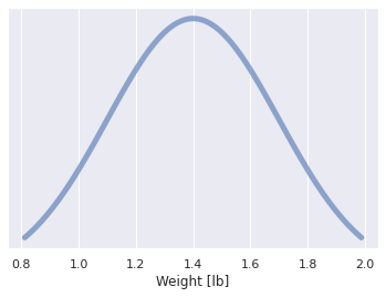
Fig. 7 Estimated distribution of bread weight with a 95% confidence interval, assumes a normal distribution of \(\mu=\) 1.4 and \(\sigma=\) 0.3 . ¶

Wait! Where is the y-axis??

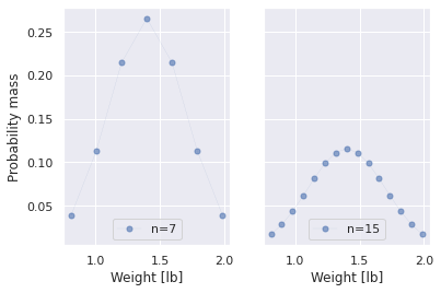
You might have noticed that Fig. 7 has no y-axis. This is intentional, and is common when showing probability distributions. A probability density function (PDF) like the one shown above is a continuous function. Reasoning about a PDF requires calculus. For those of us allergic to calculus, there is a discrete alternative, the probability mass function (PMF) . Everything beyond this point will be a PMF. When using a PMF each discrete point is assigned a bit of probability mass. The more mass a point has, the more likely the outcome that it represents will occur. Taking the normal distribution from Fig. 7 , it can be converted into a PMF in Fig. 8 using a few discrete points in the range of \([0.8,2.0]\) . The first panel uses 7 discrete points spread across the range of \([0.8,2.0]\) to represent (roughly approximate) the normal distribution, while the second panel uses 15 discrete points to represent the same distribution. In each panel the sum of the probability mass for all probability points sums to 1.0. So the more discrete points you use, the less mass any one probability point will have. This is why both panels represent the same distribution, but the distribution on the left is taller . The standard solution process was designed to skirt around the problem of normalizing distributions to have a total probability mass of 1.0, so this is more than just a nuance of using distributions and Bayes theorem.

When comparing two PMF’s, it helps to use the same number of points. In general, you are just interested in the shape of the distribution and what range of possible values the distribution is over. If you use a grid method, then the probability mass values become more meaningful because they are used in our calculations.

Fig. 8 Two approximations of the PDF shown in Fig. 7 . Both panels are discrete approximations - or PMF’s - of a normal distribution with \(\mu=\) 1.4 and \(\sigma=\) 0.3 . The only difference between the panels is on the left 7 discrete points were used, while on the right 15 points were used. ¶

A special case of a probability distribution is the probability of a probability. For example, instead of saying you believe the probability of making a sale to a customer that visits your website is 0.1, you could instead give a range of values to the probability of making a sale, in this case using the beta distribution as shown in Fig. 9 . It turns out that the beta distribution is a special case where the math works out easily when using Bayes theorem, which is why we use it here.

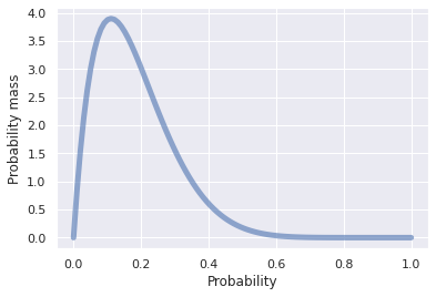
Fig. 9 Example of a beta distribution with \(\alpha=\) 2 and \(\beta=\) 9 . ¶

The Beta distribution is defined as:

\[Beta(p;\alpha,\beta) = \frac{p^{\alpha-1}(1-p)^{\beta-1}}{beta(\alpha,\beta)}\]

In this definition:

\(p\) is the random variable, or in our example the probability of a probability
\(\alpha\) and \(\beta\) are parameters that define the shape of the distribution. These are analogs to the mean and standard deviation for a normal distribution. See Fig. 10 for the many different shapes that the beta distribution can generate when utilizing different combinations of \(\alpha\) and \(\beta\) .
In the denominator \(beta(\alpha,\beta)\) , with a lowercase ‘b’, is the beta function. Confusingly \(Beta(p;\alpha,\beta)\) , with an upper case ‘B’, is the Beta distribution. I highly suggest you always use a computer to generate your Beta distributions because the beta functions is not easy to understand and itself is defined with even more complex functions. Intuitively you can consider the beta function as a normalizing factor for the Beta distribution .

Keeping all the big ‘B’ betas, little ‘b’ betas, and the greek ‘ \(\beta\) ’ parameter straight in the Beta distribution is a mess 6 . In practice, you just need to know what your \(\alpha\) and \(\beta\) parameters are, then you plug them into a computer to get your distribution. The beta distribution is a very versatile distribution. Fig. 10 shows some of the common shapes of the distribution.

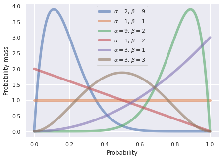
Fig. 10 Example of different shapes the beta distribution can have given different values of \(\alpha\) and \(\beta\) . ¶

Without any kind of proof 7 , I will state that Bayes theorem can be applied to the Beta distribution in the following manner:

(10) ¶ \[ Beta(p; \alpha_{post},\beta_{post}) = Beta(p;\alpha_{prior} + \alpha_{like},\beta_{prior} + \beta_{like} ) \]

The simplicity is astounding. By simply using addition, you can use Bayes theorem when your uncertainty is described with a beta distribution. The drawback is that the beta distribution only applies in the range of \([0,1]\) . So the beta distribution is a good choice for the probability of success or rates. It might be a bad choice for discrete quantities, like your estimate of the circumference of the earth in kilometers 8 .

Pretend for example that you write a book about Bayes theorem and open an online store to sell your book. After the first ten visitors to your online store, you sell one book! This is an outstanding visitor to customer conversion rate for an online product, and you begin to think that you might be headed for an early retirement. Set your priors to be \(\alpha_{prior} =\) 1 and \(\beta_{prior}=\) 9 to represent one sale and nine visitors that left the site without a purchase respectively. It turns out that your initial sale was to your mother. While she is very proud of you, she goes on to use your book to raise up her computer monitors. Out of your next 100 visitors you only sell 3 books. Your likelihoods are \(\alpha_{like} =\) 3 and \(\beta_{like}=\) 97 . Update your parameters using equation (10) with this new information by adding the prior and likelihood parameters. Therefore \(\alpha_{post} =\) 1 \(+\) 3 \(=\) 4 and \(\beta_{post}=\) 9 \(+\) 97 \(=\) 106 . Fig. 11 shows the prior, likelihood, and posterior distributions. For the sake of comparison all three distributions are shown together in one plot in Fig. 12 . The likelihood and posterior distributions are very narrow, so Fig. 12 has a truncated x-axis that makes seeing the distributions easier.

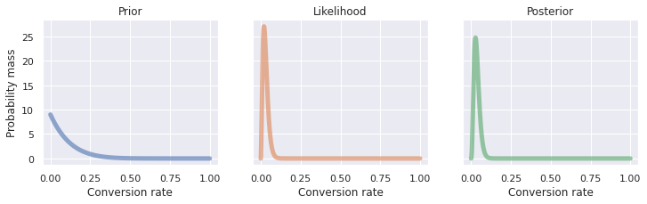
Fig. 11 Prior, likelihood, and posterior distributions for the customer conversion rate problem. ¶

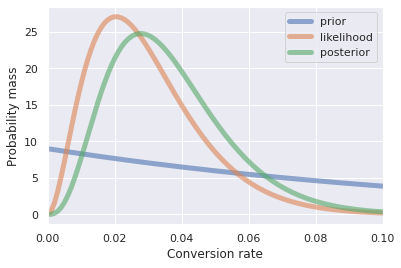
Fig. 12 Prior, likelihood, and posterior distributions plotted together for comparison. Note that the x-axis has been truncated to make the spread of the distributions easier to visualize. ¶

Distributions provide lots of advantages when quantifying uncertainty, but they can be hard to compare and analyze when either:

The shapes of the distributions are very different
The distributions are very similar to each other

The mean, \(\mu\) , of the beta distributions is not a complete description of the distribution, but is convenient for quickly comparing two distributions.

\[ \mu = \frac{\alpha}{\alpha+\beta}\]

Table 36 compares the means of the distributions shown in Fig. 12 so you can get a feel for what the posterior distribution implies about your customer conversion rate at your online book store.

Table 36 A comparison of the means of the prior, likelihood, and posterior distribution. ¶
Distribution	Mean ( \(\mu\) )
Prior	0.10
Likelihood	0.03
Posterior	0.04

This new data seriously downgrades your expectations for profit. Maybe there are not as many readers interested in Bayes theorem as you initially thought, better not quit your day job yet…However, you can see Bayes theorem in action. The prior was overly generous. The likelihood showed that in truth the conversion rate was much lower. Finally, the posterior is a compromise between the prior and the likelihood. The likelihood had many more data points than the prior, so the strength of evidence made the posterior distribution much closer to the likelihood than the prior.

The beta distribution is an example of parameter estimation with Bayes theorem. Like most things in this manual this is a special case where the math is much easier than the general case. In this manual, easy is defined as ‘easy if you have a good scientific computing environment setup’. Some examples of such an environment are python 9 , R-project 10 , or Matlab .

A/B testing ¶

Most introductory statistics classes teach null hypothesis significance testing where you can state things like, “drug A increases survival compared to the control group, p < 0.05, n = 30”. The goal of significance testing is to not trick yourself because you happened to observe a few lucky observations.

Getting null hypothesis testing correct can be onerous. Thankfully, there is not a direct analogy in Bayesian statistics for null hypothesis significance test. However, running an A/B test can answer similar questions when using Bayesian statistics.

Back to the example of the online store. Your conversion rate is rather low. To make more money, you would like to increase your conversion of site visitors to paying customers. Writing a better book is difficult and time consuming. Instead, you surmise that readers interested in Bayes theorem are likely nerdy and lonely individuals, so you update the cover of your book to include an attractive couple in swim suits (sex sells!).

After updating your book cover art, you observe how many sales you make and how many site visitors you had. Collecting this data takes time, and you are impatient, so you wait until you have just one more sale. If the original book cover design is taken as variant A, and the new sexy design is taken as variant B, then Table 37 summarizes the before and after results for your book cover redesign.

Table 37 Summary of sales for the A and B versions of your book. ¶
Version	Sales	Site Visitors
A: Original	4	110
B: Sexy	1	21

Fig. 13 shows the distributions resulting from the sales data for the two variants. Note that the x-axis has been truncated to focus on the relatively small conversion rates for both variants. A comparison between the two distributions may not be immediately obvious because the two distributions are different shapes. It is also important to note that the number of samples for each variant is very different. Variant A has 110 \(-\) 21 \(=\) 89 more samples than variant B.

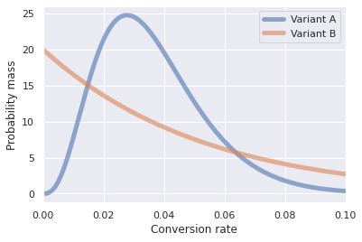
Fig. 13 Distributions for the conversion rate for both variants. ¶

Table 38 extends Table 37 with the mean values of each distribution. Based on the means of the distribution variant B is slightly better. If you only looked at the means you might conclude that variant B is better than variant A. The shapes of the distributions are neither similar or symmetric, so drawing any conclusions exclusively from the means ignores all the information about the uncertainty encoded in each distribution.

Table 38 Summary of sales and mean values for the A and B versions of the book. ¶
Version	Sales	Site Visitors	Mean ( \(\mu\) )
A: Original	4	110	0.04
B: Sexy	1	21	0.05

To get more insight into the relative merits of our book cover variants, we have to run a Monte Carlo simulation. The simulation goes like this:

Draw a random sample from the \(Beta(\alpha=\) 4 \(,\beta=\) 106 \()\) distribution that represents variant A, call it a.sample
Draw a random sample from the \(Beta(\alpha=\) 1 \(,\beta=\) 20 \()\) distribution that represents variant B, call it b.sample
Divide b.sample by a.sample and save the result as ratio
Repeat this process thousands of times and store the results in an array

Fig. 14 shows the raw data from 10,000 Monte Carlo trials, and Fig. 15 shows the results of the Monte Carlo simulation. Any simulation where the ratio of b.sample to a.sample is greater than one implies that the sexy book cover (variant B) is superior to the original cover (variant A). Again, it might not be obvious because of the spread of the data, but b.sample > a.sample in 50.18 % of the simulations.

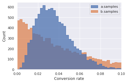
Fig. 14 Raw data for 10,000 samples drawn from each \(beta(p;\alpha,\beta)\) distribution for the Monte Carlo simulation. Note the approximate similarity to Fig. 13 because the Monte Carlo simulation is an numeric approximation of those distributions. ¶

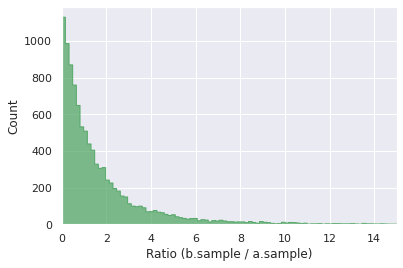
Fig. 15 Results of the Monte Carlo simulation. For each Monte Carlo trial the ratio is calculated as b.sample/a.sample . Ratio’s greater than one imply that variation B is better. ¶

If we desire to know how much better the B variant is than the A variant then we can calculate an empirical cumulative distribution function (ECDF) from our simulated data. To explain what an ECDF is, I need to first explain what a regular cumulative distribution function (CDF) is. If our probability density function for a random variable, \(t\) , is defined as a continuous function \(f(t)\) , then the CDF, denoted as \(F(x)\) is:

\[F(x) = \int_{-\inf}^{x}f(t)dt\]

\(F(x)\) represents the probability that the random variable \(t\) takes on a value less than or equal to \(x\) .

The empirical CDF is simply an approximation when \(F(x)\) is not continuous. For a value \(t_k\) , which takes on \(k\) discrete values, the empirical cdf \(\hat{F}(x)\) is the sum of the values less than or equal to \(x\) .

\[ \hat{F}(x) = \sum_{t_k \leq x} p(t_k) \]

Fig. 16 shows the empirical CDF from the Monte Carlo simulation. This plot can make reasoning about the relative merits of each variant easier. Reading off the plot for a ratio of 1.0, the ECDF is roughly 0.5. This implies that about half of the cumulative probability mass is less than a ratio of 1.0 and the other half is above 1.0. Technically, it is a 50.18 % to 49.82 % split, but that might change if we let the experiment run longer and used more data points. I would have been hard pressed to identify that from Fig. 16 because the distribution is not symmetrical like a normal distribution. In practice, this means that given the data that we have at this current time, there is no practical benefit to variant B over variant A. If we collected more data this might change, but currently changing the cover art to include sexy swimsuit models didn’t have a significant effect on our estimated conversion rate.

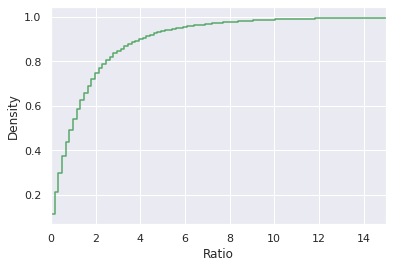
Fig. 16 Empirical cumulative distribution function for the ratio of b.samples to a.samples in the Monte Carlo simulation. ¶

Casting model comparison as parameter estimation ¶

This manual focuses almost exclusively on the model comparison form of Bayes theorem. The alternative parameter estimation approach was superficially introduced with the Beta distribution so an advanced reader would at least know there were other ways to use the theorem. Model comparison and parameter estimation are basically two sides of the same coin. This section shows a numerical approximation that uses the familiar model comparison methods to perform a type of parameter estimation calculation. Per the usual for this manual, this is not a mainstream solution method for Bayes theorem. Instead, it is intended to be instructive in how the two methods are related to each other. If you want a computationally light weight way to express your beliefs as probability distributions without having to learn more advanced numerical methods, this section might also be helpful.

In this manual, model comparison has used point estimates to quantify uncertainty, and parameter estimation has used probability distributions. This section describes what is known as a ‘grid method’ and is a hybrid of the two paradigms.

Assume that you are trying to decide if you are being cheated during a game of flip the coin 11 . The game goes something like this:

You and a friend each place a one dollar bet at the start of each round of play
Your friend flips a coin
If the coin lands heads side up your friend wins the round and collect the money for that round
If the coin lands tails side up you collect the money
Play continues until one person decides to call it quits

You are using the coin your friend brought for this game. After observing the sequence HHHHT - where ‘H’ represents the coin landing heads up and ‘T’ represents the coin landing tails up - you begin to wonder if you are being cheated, or if you are just suffering an unlucky streak. So far you have lost three dollars.

In mathematical terms, you are wondering if the coin is biased. In this context, fair implies that the coin lands on heads with a probability of 0.5. If the coin is biased the long run probability of observing heads on any toss would be some other probability - most likely a cheater would use a coin with a probability of heads significantly higher than 0.5.

The simplest unfair coin would have heads on both sides of the coin. This is obviously not the case in your current game because you have observed heads to tails in a ratio of 4:1. If the goal is to separate you from your money, your friend would want to choose a coin that is slightly unfair so you would not suspect the cheat and instead would think you are unlucky. Denote the long run bias of the coin with the parameter \(\theta\) . You don’t know what the value of \(\theta\) is, but you assume that for a coin it would be a constant. You think that the three most likely scenarios would be a coin that is biased towards heads, fair, or biased towards tails. Assign probabilities for each hypothesis:

\(p(\theta=0.25) = 0.1\) , this is the hypothesis where heads occurs less frequently than a fair coin. This is the unusual case where your friend is using a coin that is not fair, but the bias is in your favor! This is just included for comparison in this example, because nobody would knowingly bring a coin biased against them to a betting game.
\(p(\theta=0.50) = 0.6\) , this is the hypothesis for the fair coin
\(p(\theta=0.75) = 0.3\) , this is the hypothesis that you are concerned about where your friend is cheating you by using a biased coin.

Your choice of the levels 0.25, 0.50, 0.75 for \(\theta\) are arbitrary. You could choose different levels and/or a different number of levels. We chose only three values of \(\theta\) to keep things simple (see below for an expanded example with more levels). You figure that a bias of more than 0.75 or less than 0.25 would be overly suspicious so they are not considered. With a probability distribution, your belief is quantified by both the values you assign probability to, as well as the values you do not assign any probability to 12 .

The \(\theta\) parameter represents the probability of observing heads on any flip. The probability of observing tails is therefore \(1-\theta\) . The probability of observing the sequence HHHHT is:

(11) ¶ \[ p(H,H,H,H,T:\theta) = \theta \times \theta \times \theta \times \theta \times (1-\theta) \]

The colon ‘:’ in equation (11) indicates that \(\theta\) is a parameter whose value can vary. In our case \(\theta\) is restricted to the range [0,1]. The computation of the prior and posterior for each value of \(\theta\) occurs just like in the standard solution process , with an added step to ensure the posterior distribution is a proper distribution where the probability of all possible outcomes sums to 1.0.

The likelihood for each \(\theta\) is calculated by plugging the respective bias into equation (11) . For example, \(p(H,H,H,H,T|\theta=0.25) = 0.25 \times 0.25 \times 0.25 \times 0.25 \times 0.75 =\) 2.93e-03 . Table 39 shows the calculation for each value of \(\theta\) , and the distributions are shown in Fig. 17 . It is recommended to use a spreadsheet to help keep the calculation organized.

Table 39 A summary of the calculation for the posterior probability distribution of the biased coin after observing HHHHT. ¶
\(\theta\)	0.25	0.5	0.75	Sum
Prior	0.10	0.60	0.30	1.00
Likelihood	2.93e-03	3.12e-02	7.91e-02	1.13e-01
Prior x Likelihood	2.9e-04	1.9e-02	2.4e-02	4.3e-02
Posterior	0.01	0.44	0.55	1.00

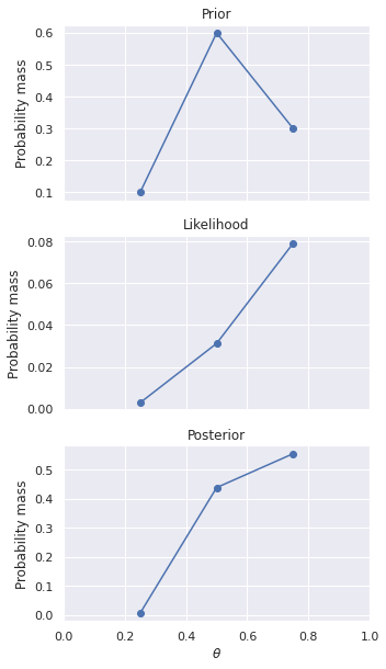
Fig. 17 Probability distribution for the bias of a coin after seeing HHHHT. ¶

As a result of this calculation, your prior beliefs have been revised by the likelihood of the observed data. Your observations so far indicate that \(\theta=0.75\) is the most likely bias for the coin, but \(\theta=0.5\) still has significant probability as well. The only thing you can say definitely at this point is you do not believe the bias of the coin is in your favor.

The sum of each row is included to highlight how and when normalization is required. The prior distribution sums to one, and, therefore, is a proper probability distribution. The likelihood does not sum to one. This is expected because the likelihoods only need to be accurate relative to each other. The \(prior \times likelihood\) step is an intermediate calculation. The sum of the \(prior \times likelihood\) for all values of \(\theta\) is used as the normalizing factor to calculate the posterior. For each value of \(\theta\) , the posterior is calculated as:

\[posterior = \frac{(prior \times likelihood)}{\sum(prior \times likelihood)}\]

The normalizing constant in the denominator makes the posterior a proper distribution that sums to one. While crude, and limited in application, this is a rudimentary way to perform parameter estimation using the methods described in this manual. The more complex forms of Bayes theorem include a normalizing constant that is more rigorously defined (using an integral, see equation (6) ). In the standard solution process we sidestep the calculation of the normalizing constant by using relative odds.

The grid method is an approximate numerical method. Using a finer grid may be beneficial in some use cases. For example, the same problem above can be refined by using a finer grid. Table 40 shows the same calculation using a finer grid, and the distributions are shown in Fig. 18 . As the grid starts to contain more points, it would be customary, but not strictly required, to set your prior distribution with a commonly used distribution, such as the normal or beta distributions. Note how in the previous example shown in Table 39 , the prior was neither symmetric or taken from a distribution of any kind. Mathematically, any distribution is valid, but when you start using a finer grid it might become more convenient to use a known distribution so each prior does not have to be set manually.

Table 40 A summary of the calculation for the posterior probability distribution of the biased coin after observing HHHHT on a finer grid than previously shown in Table 39 / Fig. 17 . ¶
\(\theta\)	0.1	0.2	0.3	0.4	0.5	0.6	0.7	0.8	0.9	Sum
Prior	0.05	0.08	0.12	0.16	0.17	0.16	0.12	0.08	0.05	1.00
Likelihood	9.0E-05	1.3E-03	0.01	0.02	0.03	0.05	0.07	0.08	0.07	0.33
Prior x Likelihood	4.3E-06	1.1E-04	7.1E-04	2.4E-03	0.01	0.01	0.01	0.01	3.1E-03	0.04
Posterior	1.2E-04	3.0E-03	0.02	0.07	0.15	0.23	0.25	0.19	0.09	1.00

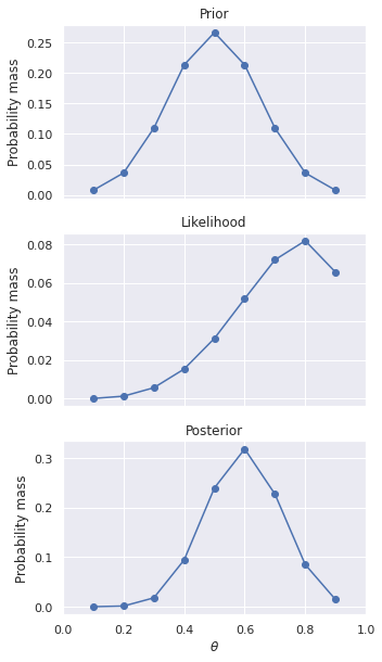
Fig. 18 Probability distribution with a finer grid for the bias of a coin after seeing HHHHT. ¶

Using a finer grid reveals a couple of different things. The probabilities for all the values of \(\theta\) have been reduced because you are considering more possible states of the coin. Also, the prior has been changed so the results can not be directly compared to Table 39 . Lastly it seems more likely that the coin is biased. The cumulative probability that \(\theta>0.5\) is now 0.65 .

While concerned about the fairness of the coin based on the results in Table 40 , the risk of accusing your friend of cheating is too great, so you continue with five additional rounds which results in the sequence HHTHH. Your total loss at this point is six dollars. The results of updating your beliefs with this new sequence is shown in Table Table 41 , and the distributions are visualized in Fig. 19 .

Table 41 An update to the posterior probability distribution using Bayes theorem shown in Table 40 / Fig. 18 after observing a new sequence of HHTHH. ¶
\(\theta\)	0.1	0.2	0.3	0.4	0.5	0.6	0.7	0.8	0.9	Sum
Prior	0.00	0.00	0.02	0.09	0.24	0.32	0.23	0.09	0.01	1.00
Likelihood	9.00e-05	1.28e-03	5.67e-03	1.54e-02	3.12e-02	5.18e-02	7.20e-02	8.19e-02	6.56e-02	3.25e-01
Prior x Likelihood	1.8e-09	1.7e-06	1.0e-04	1.5e-03	7.5e-03	1.7e-02	1.6e-02	7.0e-03	9.4e-04	5.0e-02
Posterior	0.00	0.00	0.00	0.03	0.15	0.33	0.33	0.14	0.02	1.00

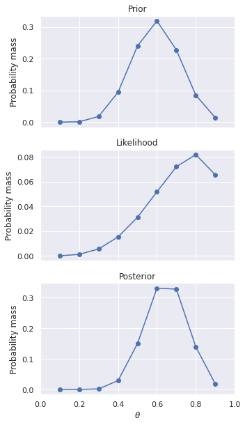
Fig. 19 Probability distribution with a finer grid for the bias of the coin after seeing an additional HHTHH. ¶

After this update, the peak of the probability distribution is clearly not centered over \(\theta=0.5\) anymore, but instead at a value of \(\theta\) that biases the coin in favor of your friend. The cumulative probability of \(\theta>0.5\) is now 0.82 .

The math is indicating that you are being cheated, but decision making is more complex than just looking at the output of Bayes theorem. You will potentially lose a friend and start a fight if you declare, based on 10 flips of a coin, that he is cheating. The field of decision theory considers the penalty of making an incorrect decision and helps you optimize your choices. Decision theory is beyond the scope of this manual, but the principle of being humble with your uncertainty applies here. The output of Bayes theorem depends heavily on the prior. What if you had chosen a different prior? Table 42 assumes a uniform prior where each value of \(\theta\) is given an equal probability. This means that every value is equally likely - or you have absolutely no opinion about the possible outcomes in advance. Having absolutely no opinion seems doubtful, but this is considered the most naive prior you can set. Unfortunately, for your friend, the results when using a uniform prior are more damming than your initial calculation (see Table 41 for comparison). Your choice of a prior has potentially impacted your decision making.

Table 42 A repeat of the calculation in Table 41 / Fig. 19 using Bayes theorem with a uniform prior. This calculation reflects observing 8 heads and 2 tails. ¶
\(\theta\)	0.1	0.2	0.3	0.4	0.5	0.6	0.7	0.8	0.9	Sum
Prior	0.11	0.11	0.11	0.11	0.11	0.11	0.11	0.11	0.11	1.00
Likelihood	0.00	0.00	0.00	0.00	0.00	0.00	0.01	0.01	0.00	0.02
Prior x Likelihood	9.0e-10	1.8e-07	3.6e-06	2.6e-05	1.1e-04	3.0e-04	5.8e-04	7.5e-04	4.8e-04	2.2e-03
Posterior	0.00	0.00	0.00	0.01	0.05	0.13	0.26	0.33	0.21	1.00

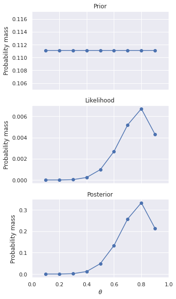
Fig. 20 Probability distributions with a uniform prior after seeing HHHHT. ¶

You can choose a prior that would make your friend look less guilty of cheating. Manufacturing a biased coin that looks indistinguishable from a standard coin would be very difficult to achieve. Maybe your prior should place a higher probability on \(\theta=0.5\) and assign minimal probability to the other values of \(\theta\) ? Table 43 and Fig. 21 shows a result that is gives significant probability to the coin being fair and potentially saves your friendship.

Table 43 A repeat of the calculation in Table Table 41 with a normal distribution ( \(\mu=0.5\) , \(\sigma=0.05\) ). This calculation reflects observing 8 heads and 2 tails. ¶
\(\theta\)	0.1	0.2	0.3	0.4	0.5	0.6	0.7	0.8	0.9	Sum
Prior	0.00	0.00	0.00	0.11	0.79	0.11	0.00	0.00	0.00	1.00
Likelihood	0.00	0.00	0.00	0.00	0.00	0.00	0.01	0.01	0.00	0.02
Prior x Likelihood	8.1e-23	2.0e-14	8.5e-09	2.5e-05	7.7e-04	2.9e-04	1.4e-06	8.0e-11	4.3e-17	1.1e-03
Posterior	0.00	0.00	0.00	0.02	0.71	0.26	0.00	0.00	0.00	1.00

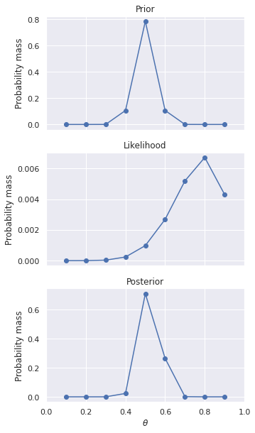
Fig. 21 Probability distribution with a finer grid for the bias of a coin after seeing HHHHT. ¶

Given the same data, three different results can be achieved by choosing a different prior. This begs the question, which prior is more appropriate? Well, unfortunately, it depends on your specific circumstance and how/if you plan to take an action based on your beliefs. Again, when using subjective probabilities your results are personal. The data suggests that the coin is biased. Your selection of a prior determines how much influence the data should have when revising your beliefs. A tight narrow distribution around \(\theta=0.5\) like in Fig. 21 implies that your beliefs will not be influenced by the data very much. On the other extreme, a uniform prior, like Fig. 20 , implies that your beliefs will be only informed by the data. Setting a prior will certainly be difficult when you have a vested interest (your friendship) in the posterior belief.

As a final note, if you take the resolution of the grid to be very fine your results will start looking like continuous distributions. For example, Fig. 22 reproduces Fig. 19 with 10 times more points on the grid. In general, more points are better, which should eventually lead to using a more powerful numerical method. The method shown here is basically a brute force approach. See the references for more sophisticated solutions.

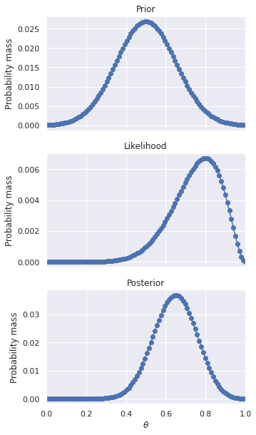
Fig. 22 Probability distribution with a finer grid for the bias of a coin after seeing HHHHT. ¶

Per the usual, with Bayes theorem your results are personal and you should be realistic about the uncertainty and bias of your reasoning. The grid method may be a way to improve your reasoning over using simple point estimates, but comes with the penalty of increased computational complexity. Grid methods show how model comparison and parameter estimation seem different, but are actually related methods.

Summary ¶

This appendix sampled a number of unique or complex techniques associated with Bayes theorem that were not included in the main text of the manual. The manual aims to be self contained for a very narrow, but useful, application of Bayes theorem. This appendix aims to be the opposite, general and vague, to provide a jumping off point for further investigation elsewhere .

1: The Pineapples and Nordiques are pop culture references to the mid 90’s television series Pinky and the Brain .
2: Theses are characters from the board game Clue .
3: See also: Worcestershire cola example , Spam email filter , The Mony Hall problem , Heuristic for evaluating medical news for examples of multiple belief revision.
4: There is an interesting discussion on the arbital website about what constitutes extreme evidence.
5: When you flip the order you write the odds in, the odds ratios are inverted as well. In our running example \(0.996/0.005 = 199.2\) so the inverse is \(0.005/0.996 = 0.00502 = 1/199.2\) .
6: To further complicate things, not all authors use consistent nomenclature. Look up the beta distribution on wikipedia and you will see a similar, but not identical, definition compared to what is shown in this manual.
7: See Kurt or Kruschke for a formal proof.
8: The earth is not a perfect sphere, so depending on how it is measured, the circumference of the earth is reported to be in the range of 40,008 to 40,075 km ( source ).
9: A new user should start with an installer that includes python along with a development environment and all the scientific computing libraries pre-installed. See winPy or anaconda for good staring points.
10: A new user should start with the instructions for installing the free RStudio development environment which makes using R much more user friendly.
11: When I started writing this manual, I decided to omit all card, dice, and coin examples because I believe they are not very representative of practical real life problems . It is really hard to give examples of ‘probability of a probability’ scenarios without using the biased coin example described here because it is the simplest example. I justify this betrayal of my initial stated goal to myself by burying this example in the depths of a chapter that I discourage readers from using 😂.
12: Some authors use the idea, or analogy, of probability mass to describe this process of describing your beliefs as a distribution. Imagine that you have a ball of modeling clay and are asked to quantify your beliefs about some proposition by laying clumps of mass onto a row of plates that represent a probability index. For example, will it rain today? You are given a row of plates which represent 0.1 increments of belief. The first plate is labeled 0.0, the next 0.1, and so on until the last plate which represents 1.0. To assign probability mass in accordance to your beliefs, you break off chunks of modeling clay and lay them on the plates. The mass you place on any one plate indicates your belief in that value. A key point here is that you are limited to only using clay from the initial ball you were given to describe your beliefs, and can only distribute clay to the existing plates. If you use more plates, to provide finer resolution of your beliefs, you are still restricted to the one ball of clay. If all plates are given equal mass then the probability distribution is ‘uniform’. If some plates have more mass then others then you have indicated that you think some outcomes are more likely than others. Plates assigned no mass are essentially not being considered as a possible outcome. When using Bayes theorem, the difference between very little probability mass and absolutely no mass is important. If your prior assigns no mass to a particular outcome then your prior will never include that outcome. Strictly speaking, a probability distribution is a continuous function, while a probability mass function is a discrete function with a finite number of ‘plates’ that can have mass assigned to them.

Bayes Theorem - The Missing Manual

Appendix: Theory ¶

Disambiguation of the language we use for probability and statistics ¶

Derivation of Bayes Theorem ¶

Probability notation ¶

Basic notation ¶

Product rule of probability ¶

Marginal probability ¶

Mutually exclusive and exhaustive propositions ¶

The special case of binary events ¶

Probability form of Bayes theorem ¶

Application specific notation ¶

Probability of the evidence ¶

Temporal sequencing ¶

Odds notation ¶

A very brief history of odds and gambling ¶

Relative odds ¶

Odds form of Bayes theorem ¶

Revisiting the mystic seer example ¶

Log odds form ¶

The interplay between the prior and the relative likelihood ¶

Extreme relative likelihoods ¶

Extreme priors ¶

Examples of alternative forms of Bayes theorem ¶

Pink shirts ¶

Two boys in the family example ¶

Three hypothesis and the probability form of Bayes theorem ¶

Three hypothesis and a normalization factor ¶

Three hypothesis and the odds form of Bayes theorem ¶

One hypothesis and the probability form of Bayes theorem ¶

Comparison of results for the two boys problem ¶

Other applications ¶

Beta distribution ¶

A/B testing ¶

Casting model comparison as parameter estimation ¶

Summary ¶