Bayes theorem solution process 
The quintessential example for introducing Bayes theorem is a medical diagnostics test. This example from Eliezer Yudkowsky is a classic. It explains why the example is attention grabbing:
1% of women at age forty who participate in routine screening have breast cancer. 80% of women with breast cancer will get positive mammographies. 9.6% of women without breast cancer will also get positive mammographies. A woman in this age group had a positive mammography in a routine screening. What is the probability that she actually has breast cancer?
Next, suppose I told you that most doctors get the same wrong answer on this problem - usually, only around 15% of doctors get it right. See Casscells, Schoenberger, and Grayboys 1978; Eddy 1982; Gigerenzer and Hoffrage 1995; and many other studies. It’s a surprising result, which is easy to replicate, so it’s been extensively replicated.
— Source
We will return to the quintessential example described above later in this chapter. To illustrate the process for solving problems with Bayes theorem, we will solve the same type of problem using convenient round looking numbers to make things easy. There are many ways to solve problems, but for the sake of consistency, we will use this standard approach over and over in this manual.
Let’s use a similar medical example from arbitral.com :
“Suppose you are a nurse screening incoming freshmen for diseasitis. Last year 20% of incoming students had diseasitis. During the screening test students place a tongue depressor into their mouth. If the tongue depressor turns black, the student may have diseasitis.
Among the students with diseasitis, 90% turn the tongue depressor black
Because the tongue depressor test is very cheap and quick to administer, 30% of students who are healthy also turn the tongue depressor black.
If you have a student that turns the tongue depressor black, what is the probability that they have diseasitis?”
Multiple studies show that thinking about concrete numbers such as “20 out of 100 students” is more likely to produce correct spontaneous reasoning on these problems than thinking about percentages like “20% of students” 1 , so that will be our starting point. Imagine a group of 100 incoming freshmen, 20 of them would have diseasitis. See Fig. 1 for a visual representation of this situation.
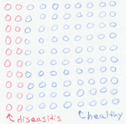
Fig. 1 Diagram representing 100 students. Red circles represent incoming students sick with diseasitis. Blue circles represent healthy students. 
Of the 20 students with diseasitis, the tongue depressor would turn black for 90% of them. In our example 18 out of the 20 sick students would be identified as sick with a black tongue depressor. Of the healthy students, 30% of them would turn the tongue depressor black despite being healthy. In our example 24 of the 80 healthy students would test positive for diseasitis even though they were sick. Fig. 2 shows an updated diagram with the respective positive tests from the sick and healthy groups.
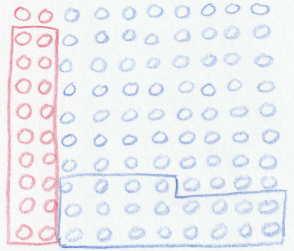
Fig. 2 Positive tests in both the sick and healthy portions of the incoming students. 
There are a total of \(18+24=42\) students that turn the tongue depressor black, but only 18 of them are actually sick. Therefore your odds of being sick given that you turned the tongue depressor black are 18:24 - simplifies to 3:4, or about \(18/(18+24) \approx 0.43\) probability of being sick. See Fig. 3 for a visual representation of the results. This result can be a bit counter intuitive because the test is correct 90% of the time. There were relatively few cases of diseasitis to begin with, which makes the odds of actually having the disease much lower than the 90% true positive rate reported for the test.
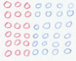
Fig. 3 Relative odds of sick to healthy students 
Standardized example 
In future examples we will forgo drawing all those little circles and use a simple box to describe our proportions. Here is the same problem using the soon to become standard format:
Evidence: A student turns a tongue depressor black.
Question: What do you believe the odds are that the student is sick with diseasitis?
Hypothesis: Establish two hypothesis to describe the two possible states of the student.
-
\(H_1\) : The student is sick with diseasitis
-
\(H_2\) : The student is healthy 2
For the sake of accounting represent the odds as \(H_1:H_2\) for sick:healthy. The opposite representation (healthy:sick) is equally as valid, just mind that you are always consistent with how you write your odds.
Prior: “Last year 20% of the incoming freshmen had diseasitis.”
Out of a representative group of 100 students, 20 of them would have diseasitis and the other 80 would be healthy. Set the prior odds to 20:80 which simplifies to 1:4. Draw a square and do your best to eyeball in a line that represents 1:4 odds. Label the small area ‘sick’ and the big area ‘healthy’. See Fig. 4 for a visual representation of the prior odds.
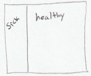
Fig. 4 Diagram representing prior odds of a student being sick with diseasitis. The region labeled sick represents 20 sick students, or odds of 1:4 for sick:healthy. 
Relative likelihood: What is the likelihood that if you make the tongue depressor black you will be sick? It depends if you are in the sick or healthy box…
-
If \(H_1\) is true then you are sick and there is a 0.9 probability you will turn a tongue depressor black. Shade in 90% of the area in the ‘sick’ box.
-
If \(H_2\) is true then you are healthy and there is a 0.3 probability you will turn the tongue depressor black. Shade in 30% of the area in the ‘healthy’ box
The relative likelihood in our example is 0.9:0.3, or 90:30, or 3:1 when simplified (see Fig. 5 ). Note that a relative likelihood is not a probability. This example intentionally shows that the likelihood does not have to sum to 1. Much like relative odds, the relative likelihood is a ratio. If your data supports both hypotheses equally well then the relative likelihood is close to one. The relative likelihood helps you quantify the strength of your evidence. Only when the evidence strongly supports one hypothesis over another does the relative likelihood revise your prior beliefs. The best data points to collect differentiates your competing hypothesis by having a relative likelihood that is far from one.
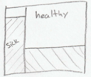
Fig. 5 Diagram representing the relative likelihood of each group showing a positive test results. The shaded region for the ‘sick’ group represents a 0.9 probability of testing positive. The shaded region for the ‘healthy’ group represents a 0.3 probability of testing positive. The posterior odds are represented by the ratio of the shaded areas. 
Posterior:
At this point you can visually inspect your diagram and get a sense for what the posterior odds are. The odds that you are sick, given that you turned a tongue depressor black, is the ratio of the two shaded areas. In our example the shaded ‘sick’ rectangle is a little bit smaller than the shaded ‘healthy’ rectangle, so the odds of being sick a a bit under 1:1, or a bit less than 0.5 probability.
If you need to, you can work out the math to get a more precise answer. See Table 3 for the complete calculation.
|
Sick |
Healthy |
|
|---|---|---|
|
Prior odds |
1 |
4 |
|
Likelihood |
3 |
1 |
|
Posterior odds |
3 |
4 |
|
Probability |
0.43 |
0.57 |
Converted back into a probability, there is a \(3/(3+4) \approx 0.43\) probability of being sick if a student blackens a tongue depressor.
The diseasitis example makes the math easy, but is not representative of most medical tests. If we work the breast cancer example shown above from Yudkowsky the probability of being sick given a positive test is considerably smaller than the diseasitis example. Results of applying Bayes theorem are shown in Table 4 .
|
Sick |
Healthy |
|
|---|---|---|
|
Prior odds |
1 |
99 |
|
Likelihood |
800 |
96 |
|
Posterior odds |
800 |
9504 |
|
Simplified posterior (approximate) |
8 |
95 |
|
Probability |
0.08 |
0.92 |
In the Yudkowsky example, the odds of being sick given a positive test are 800:9504, roughly equivalent to 8:95, or approximately a 0.08 probability of being sick. This is shocking because medical professionals reportedly struggle to correctly calculate the probability of sickness. I will however contend that their inability to properly calculate the correct answer does not imply that they lack the proper medical intuition to provide good care. As the name implies, a screening test is the first of potentially many tests that would be administered if a diagnosis of cancer is suspected. To my knowledge, there is no crisis in the medical communities treatment of cancer. This example is useful mainly for teaching Bayes theorem, not influencing the training of doctors. In my opinion, thinking with Bayes theorem is much more important than calculating a precise answer. Interestingly, the accuracy of reading mammographies has increased due to algorithms based in part on Bayes theorem 3 since the studies citing that medical professionals can’t calculate the correct answer were published.
Another interesting intersection of Bayes theorem and breast cancer screening involved a controversy in 2009 when a U.S. Government task force suggested that women should start getting mammograms to screen for breast cancer at age 50, instead of at the customary age of 40 4 . It also suggested changing the rate of screenings from every two years to every three years. The argument is that the base rate of cancer in 40 year old women is so low that the cost of false positives (healthy women with a test that seemed to indicate cancer) outweighed the benefits of the testing for the population as a whole. The downsides include radiation exposure and unnecessary treatment. As the son of a breast cancer survivor and the father of daughters, this recommendation certainly evokes an emotional response that highlights the difference between probability theory (what are the odds) and decision theory (how to use the odds to make decisions).
Standard solution process 
The standard process for using Bayes theorem throughout this article will be:
-
Identify the problem as a candidate for Bayes theorem. Usually the data arrives prior to generating a hypothesis, and you are uncertain about the underlying mechanisms generating the data.
-
Clearly state the question you are trying to answer in terms of a belief.
-
Establish two or more competing hypothesis that might explain the data you are observing.
-
For accounting purposes, decide how you will be writing the odds. For example - sick:healthy or maybe healthy:sick.
-
Identify the prior odds.
-
Establish the relative likelihood of the data occurring 5 . It may help to follow this internal prompt to establish the relative likelihoods:
-
If your first hypothesis is true, what would be the probability of observing this data?
-
If your second hypothesis is true, what would be the probability of observing this data?
-
Continue this questioning for each hypothesis.
-
Then, take the ratio of the probabilities as your relative likelihood. Don’t worry if they don’t sum to 1.
-
-
Calculate the posterior odds using term-by-term multiplication
If you only have two hypothesis, you can visualize the results by drawing a diagram:
-
Start by drawing a square to represent the entirety of the probability space.
-
Set your priors, then draw a vertical line to divide the square into two areas proportional to your prior odds. If the prior odds of \(H_1:H_2\) are 1:4 then imagine dividing the square into 5 equal vertical parts, then draw a line that divides the space into a segment of one and a segment of four.
-
Set your relative likelihoods. Shade each respective part to show the likelihood of the data given the hypothesis. If your relative likelihood is 0.9:0.3 = 9:3 = 3:1 then shade 90% of the area that represents \(H_1\) and 30% of the area that represents \(H_2\) .
-
The posterior odds are represented by the ratio of the shaded areas.
With a mathematical form of \(a \times b = c\) , there are only a couple different ways you can get Bayes theorem wrong. The most likely routes to failure are:
-
Math error - simply failing to define the odds properly or making an arithmetic error
-
Choosing inaccurate prior odds
-
Choosing inaccurate likelihood odds
Luckily, Bayes theorem inherently handles uncertainty well. As long as your estimates of the prior odds and relative likelihood are accurate to an order of magnitude then the posterior odds are useful for decision making.
Summary 
The next chapter is dedicated to solving a large number of worked problems. This includes easy word problems to give you practice with the mechanics of using the formula and then progresses in difficulty up to seemingly intractable problems. At first everything you need to work the problem will be contained in the example. After that the problems will delve into real life scenarios. Everything hinges on your ability to pick somewhat reasonable prior odds and likelihood ratios. There is often no “right” answer to these types of problems, but probably a wrong answer. Getting a close enough answer is usually well within your abilities with a little practice, so don’t fret about that aspect.
I contend that the real power of Bayes theorem is the intuition it gives you when making decisions. Hopefully, the examples allow you to identify in your personal life problems that are candidates for using Bayes theorem.
- 1
-
For example, see “Probabilistic reasoning in clinical medicine” by David M. Eddy (1982). This claim originally came from the diseasitis article .
- 2
-
The student is healthy, or at least NOT sick with diseasitis.
- 3
-
See “Using AI to improve breast cancer screening” and the peer reviewed journal article . Also see a news article about the research for additional context with respect to other previous studies.
- 4
-
See New Clarity on Who Needs Mammograms — When for a discussion of why the changes were recommended and how they could have been communicated differently.
- 5
-
So far we have simply told you what the relative likelihood should be. In practice this wont usually be given to you. Many of the examples in this manual show how to estimate the likelihood when it is not a given.